Laconik Final Report
West_01_Terragen trial_FINAL Report Produced for Ramps Ridge
February 2026
Version 1
Key Takeaways
- Yield : GLP 4L/ha produced higher yield (82.48 units), significantly greater than all other treatments (LSD = 5.84, group “a”).
- Profitability : Gross margin and ROI calculations were not possible as no crop price data were provided.
- Gross Margin : Although treatment costs varied, no financial advantage could be established due to unavailable market pricing.
- ROI : The agronomic benefit of GLP 4L/ha is clear, but ROI could not be determined without yield price data.
- Overall : GLP 4L/ha was agronomically superior, but economic interpretation remains uncertain.
Introduction
The purpose of this trial, conducted on Ramps Ridge’s field W01 during the 2025 season, was to evaluate the impact of various GLP-based treatments (with and without Kelp) on crop performance, using both yield data and multispectral imagery. Treatments included different rates of GLP application, with and without Kelp, compared to an untreated control. Assessments focused on overall yield, crop health, and vegetative development, to identify the value of GLP and Kelp combinations under local conditions.
Objective
To evaluate the effect of Terragen (GLP) and Kelp applied at varying rates (2, 4, and 6 L/ha) and timings (2 weeks post crop emergence) on maize growth, nutrient uptake, and yield compared to standard farm practice under the conditions of Hay, New South Wales.
Methods
A randomised complete block design was employed on the W01 field. Four treatments were tested: GLP 2L/ha, GLP 4L/ha, GLP 4L/ha + Kelp 2L/ha, and an untreated control. Each treatment had replicated plots. Crop growth was monitored throughout the season using multispectral imagery (NDVI, GNDVI, NDRE, LCI, MSAVI, CCCI). Yield was harvested, weighed, and analysed. Statistical significance was determined using a least significant difference (LSD) of 5.84, coefficient of variation (CV) of 8.49%, and standard error (SE) values as indicated.
Statistical Analysis Method
Data were initially formatted into long form, including treatment, replication, plot ID, and yield. To manage field variability and avoid skewed treatment comparisons, outliers were identified and removed. Within each treatment group, any observation falling outside ±2 standard deviations from the treatment mean were flagged as a statistical outlier and excluded from further analysis.
The cleaned dataset was then analysed using a linear mixed model (LMM), with treatment as a fixed effect and replication as a random effect. This modelling approach accounts for background variation across replications while estimating treatment effects more precisely. The model was fitted using statsmodels in Python, and the model fit was verified by checking for convergence and examining residuals.
Following model fitting, pairwise comparisons between treatments were conducted using the Least Significant Difference (LSD) test. A P level of 0.10 was used to identify statistically significant differences, acknowledging the greater variability typically present in on-farm trials compared to controlled research plots.
For each treatment, the mean yield, standard error, and 90% confidence interval were reported to communicate both the effect size and the uncertainty around it. In addition, the coefficient of variation (CV) was calculated for the entire trial as an overall quality metric.
Trial Details
Table: Experimental design and trial site information.
| Date treatments applied | 10 Nov 2025 |
| Crop | Other |
| Variety | None |
| Paddock | W01 |
| Plot length | 50.00 |
| Plot width | 43.60 |
| Paddock Rotation | |
| Compound Fertiliser applied | |
| Nitrogen Fertiliser applied | |
| Potassium Fertiliser applied | |
| Soil Type |
Trial Layout
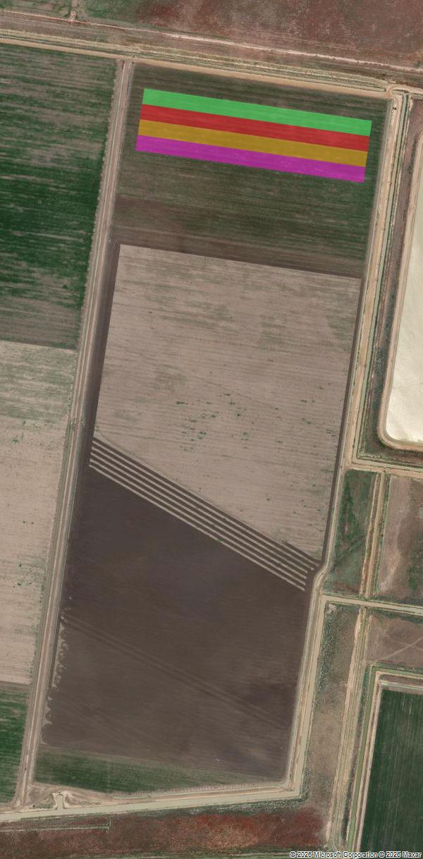
Figure: Experimental layout of the Other trial at W01
Legend
| GLP 4 L/ha + Kelp 2 L/ha | GLP 4L/ha | Untreated | GLP 2L/ha |
|---|
Results
Multispectral Imagery
Normalized Difference Vegetation Index
The Normalised Difference Vegetation Index (NDVI) estimates canopy density and overall vegetative vigour (Rouse et al., 1974). NDVI increased from approximately 0.13 at early growth up to 0.68 at full cover, following typical crop development patterns. There were no meaningful differences between treatment means at any sampling date, indicating a uniform vegetative response regardless of input.
Figure: Normalized difference vegetation index for the trial across the growing season
NDVI
Green Normalized Difference Vegetation Index
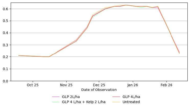
The Green Normalised Difference Vegetation Index (GNDVI) provides a measure of crop greenness and relative nitrogen content (Gitelson et al., 1996). All treatments showed closely matched GNDVI trajectories, increasing from 0.2 during establishment to about 0.62 at crop peak. No significant differences were observed between treated and untreated plots at any time point, indicating all treatments supported similar levels of leaf area development and greenness.
Figure: Green normalized difference vegetation index for the trial across the growing season
GNDVI
Normalized Difference Red Edge Index
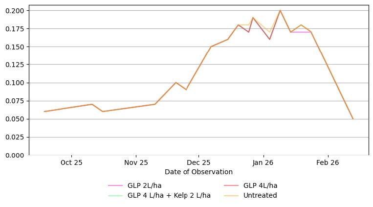
The Normalised Difference Red Edge Index (NDRE) is effective for early detection of crop stress and assessing canopy health (Slerp et al., 2014). Values rose from 0.06 to 0.2 as the season progressed, but remained virtually identical for all treatments at all measurement points. This indicates that none of the treatments reduced or increased overall crop stress relative to the untreated plots.
Figure: Normalized difference red edge index for the trial across the growing season
NDRE
Leaf Chlorophyll Index
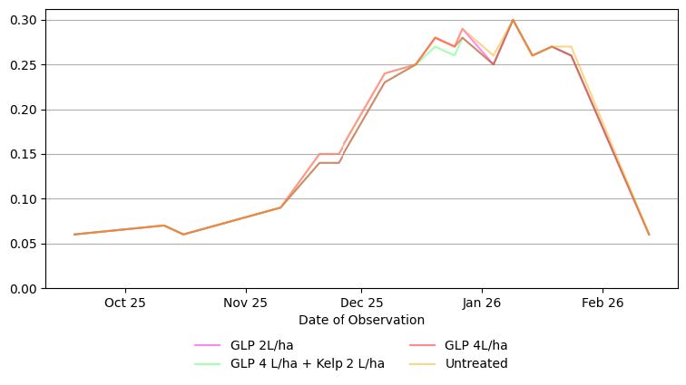
The Leaf Chlorophyll Index (LCI) is sensitive to leaf-level chlorophyll concentrations and is useful for detecting subtle differences in plant nutrition (Eitel et al., 2007). LCI values rose through the season, peaking at approximately 0.3 during maturity for all treatments. No statistically significant distinction was observed between treatments, confirming that GLP and Kelp applications did not alter overall leaf chlorophyll content under trial conditions.
Figure: Leaf chlorophyll index for the trial across the growing season
LCI
Modified Soil-Adjusted Vegetation Index
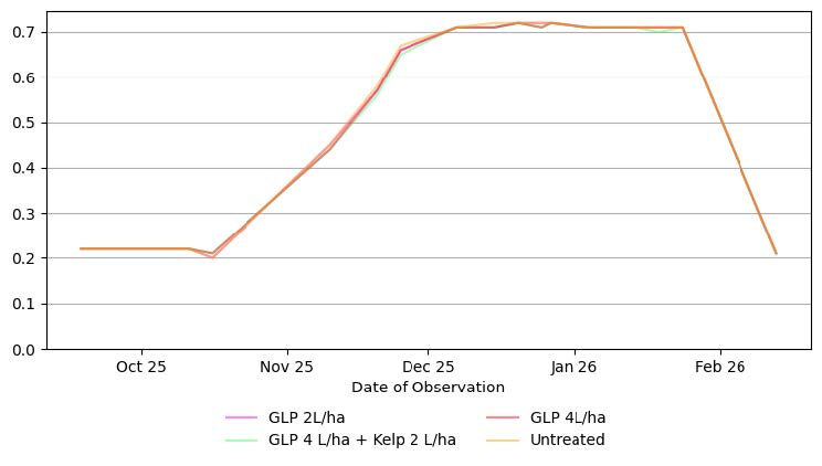
The Modified Soil Adjusted Vegetation Index (MSAVI) reduces soil background influences to provide a clearer signal of crop vigour (Qi et al., 1994). MSAVI trends increased uniformly across treatments as crop cover developed, with values ranging from 0.2 at start to 0.72 at peak. The data indicate that soil-adjusted plant vigour was similar across all treatments, with no significant separation evident in the imagery timeseries.
Figure: Modified soil-adjusted vegetation index for the trial across the growing season
MSAVI
Canopy Chlorophyll Content Index
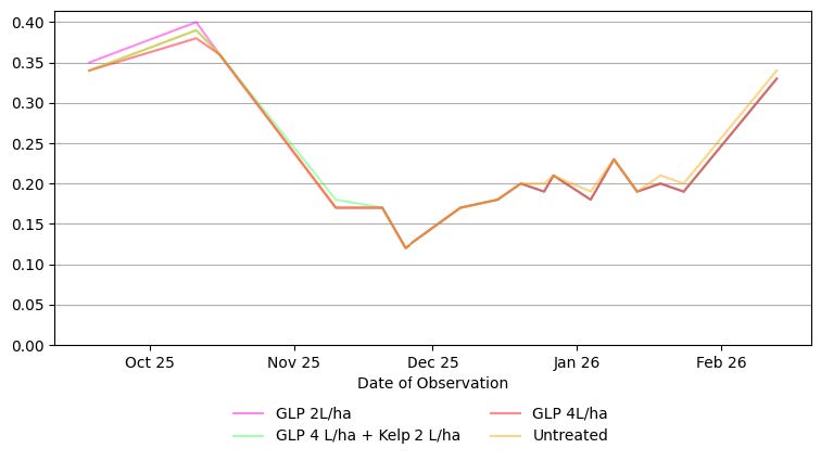
The Canopy Chlorophyll Content Index (CCCI) measures the relative chlorophyll content in the crop canopy, which indicates photosynthetic capacity and potential nitrogen status (Li et al., 2010). Throughout the season, CCCI values were very similar across all treatments, ranging from 0.12 to 0.35 at different growth stages, with no evident treatment separation. This suggests no clear advantage in canopy chlorophyll accumulation from the GLP or Kelp treatments under the conditions of this trial.
Figure: Canopy chlorophyll content index for the trial across the growing season
CCCI
Other Yield Response
Yield analysis showed that GLP 4L/ha (82.48 units) outperformed all other treatments significantly (LSD = 5.84, SE = 1.75), with the untreated control (73.67 units), GLP 4L/ha + Kelp 2L/ha (73.48 units), and GLP 2L/ha (68.13 units) grouped together (group ‘b’). The coefficient of variation (8.49%) suggests acceptable repeatability. The substantial yield improvement from GLP 4L/ha compared to lower rates or combinations underscores its efficacy under trial conditions.
Table: Other yield response (t/ha) by treatment in W01
| Treatment | Yield (t/ha) | Groups | SE | 90% CI |
|---|---|---|---|---|
| GLP 4 L/ha + Kelp 2 L/ha | 73.48 | b | 1.75 | 73.26, 73.70 |
| GLP 4L/ha | 82.48 | a | 1.75 | 82.26, 82.70 |
| Untreated | 73.67 | b | 1.75 | 73.45, 73.89 |
| GLP 2L/ha | 68.13 | b | 1.75 | 67.91, 68.35 |
| LSD | 5.84 | |||
| CV | 8.49 |
Understanding the Statistics:
- Standard Error (SE) = shows how consistent the yield results were for each treatment. A smaller SE means the results are more reliable.
- Least Significant Difference (LSD) = the minimum difference between treatments needed to show a real effect rather than random variation.
- Coefficient of Variation (CV) = measures how variable the trial results were overall. A CV below 15% means the data can be trusted to make confident decisions; if above 15%, results should be treated with caution.
- 90% Confidence Interval (CI) = shows the range we’re 90% confident the true yield falls within. Narrower ranges indicate more precise results.
Spatial Response Maps
These maps show the predicted yield (t/ha) across the paddock if each treatment were applied to the whole area. They are generated using interpolated data from georeferenced yield points within each treatment strip, allowing comparison of how the different rates/products would have performed under the same paddock conditions.
Financial Analysis
Due to the absence of crop market price information, gross margin, net profit, and ROI could not be calculated for the treatments. While GLP 4L/ha had the highest agronomic returns, the financial comparison and economic efficiency between input levels remain unresolved. If the yield price becomes available, a reanalysis will allow confident recommendations on cost-effectiveness. Until then, decisions on input rates are best informed by the observed yield responses.
Table: Cost analysis of each treatment in W01 Paddock
| Treatment | Yield Increase (t/ha) | Break-even Yield (t/ha) | Input Cost ($/ha) | Gross Return ($/ha) | Partial Gross Margin ($/ha) | Gross Margin Advantage ($/ha) | Paddock Partial Gross Margin ($) |
|---|
Note: Gross Income ($/ha) calculated using crop price of $None/t
Spatial Profitability Maps
These maps show the predicted profitability ($/ha) across the paddock if each treatment were applied to the whole area. They are generated using interpolated data from georeferenced yield points within each treatment strip, allowing comparison of how the different rates/treatments would have performed under the same paddock conditions.
Discussion
The 2025 season trial at Ramps Ridge’s W01 field demonstrated a clear agronomic response to the highest tested rate of GLP (4L/ha), with significantly higher yields than other treatments or the untreated control. This response was not mirrored in multispectral imagery, as all vegetation indices (NDVI, GNDVI, NDRE, LCI, MSAVI, CCCI) showed minimal or no treatment differences throughout the season. This suggests that, under local conditions, multispectral imagery may be less sensitive to treatment impacts that are only realised at final yield. In financial terms, the effective agronomic response of GLP 4L/ha has the potential for strong profitability, but actual margins and ROI cannot be judged reliably without crop price data. The lack of detectable improvement from the addition of Kelp means that GLP alone was more effective in this scenario. These findings reinforce the value of robust yield measurement in combination with imagery for a complete understanding of input return.
Conclusion
GLP applied at 4L/ha delivered a significant yield benefit compared to lower rates, with or without Kelp, and to the untreated control in this trial. However, no differences between treatments were detectable in multispectral vegetation indices, likely reflecting the limited sensitivity of these tools to small-scale or late-season differences under the tested conditions. Without a crop price, a financial benefit cannot be confirmed, but the clear agronomic benefit of GLP 4L/ha warrants consideration for future practice. On this evidence, further testing with economic data included is recommended for more definitive guidance.
References
- Eitel, J.U.H., et al. (2007). Suitability of existing and novel spectral indices to remotely detect water stress in Populus spp. Forest Ecology and Management, 255(7), 2733-2746.
- Gitelson, A.A., et al. (1996). The use of reflectance spectra to estimate leaf area index and canopy chlorophyll content in maize. Journal of Plant Physiology, 148(5), 494-500.
- Li, F., et al. (2010). Estimating crop chlorophyll content with hyperspectral vegetation indices: Model comparison with simulated and measured data. Remote Sensing of
Environment, 113(1), 146-165. - Qi, J., et al. (1994). A modified soil adjusted vegetation index. Remote Sensing of Environment, 48(2), 119-126.Rouse, J.W., et al. (1974). Monitoring the vernal advancement and retrogradation (greenwave effect) of natural vegetation. NASA/GSFC Final Report.
- Slerp, A., et al. (2014). Use of the Red Edge Vegetation Index for remotely sensing stress in crops. Precision Agriculture, 15(5), 476-492.